Introduction to Connected Component Trees
As image and video processing applications evolve, they require new approaches to improve their processing. Typically, the classical approach based on the individual pixels in a image is not adapted for applications that act on objects, or connected structures. Bio-medical or satellite imaging applications for example, can be much more efficiently dealt with if one uses an approach based on regions or on the notion of object. The latter can be defined by grouping pixels using a connectivity rule, typically defined through their spatial proximity, but also sometimes based on their intensity, or a specific property specifically defined. Over the past decade, a specific domain of Image Processing and Mathematical Morphology tools hasbeen largely developed. It relates to the use of hierarchical representations, called the connected component trees, to replace the classical pixel based approach. While a great review can be found there, a quick overview is presented here.
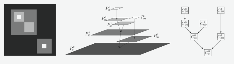
Component trees are based on the notion of connected operators, which are region-based filtering tools. They act directly on the connected components of an image, which are typically the regions where the image is constant. In images or volumes, the connected components are usually defined in terms of groups of spatially adjacent neighbors, at different threshold sets corresponding to different intensity levels. An example is given on the figure below.
Component trees are based on the notion of connected operators, which are region-based filtering tools. They act directly on the connected components of an image, which are typically the regions where the image is constant. In images or volumes, the connected components are usually defined in terms of groups of spatially adjacent neighbors, at different threshold sets corresponding to different intensity levels. An example is given on the figure below.
Credit to Michael H.F Wilkinson
The left image is a simple example of grey scale image, with different intensity levels (black being the lowest ones). In such data, processing this imaging using a region-based approach makes much more sense as it clearly consists of specific structures. As seen on the middle panel, the image can be decomposed in its flat-zones, i.e groups of pixels spatially connected at different intensity level. The hierarchical representation seen on the right is called a Max-Tree, and simply shows the image using only its connected components and the nested relations that connect them to each other. Analyzing the tree can be quickly done just by passing from branches to branches to extract for example the size of the connected components, or some specific property that they have. Filtering the image is achieved by removing a certain component from the tree, and the output image can be very simply reconstructed from the pruned tree.
Overall, these representations offer a lot of freedom, in the type of tree build, in the connectivity rule used to defined the components, in the filtering approach or also regarding the property or statistics characterizing the connected components. These tools have been successfully used in medical applications, but also in astrophysical surveys to detect very faint structures (see here). You can find below a few examples of filtering applications.
Overall, these representations offer a lot of freedom, in the type of tree build, in the connectivity rule used to defined the components, in the filtering approach or also regarding the property or statistics characterizing the connected components. These tools have been successfully used in medical applications, but also in astrophysical surveys to detect very faint structures (see here). You can find below a few examples of filtering applications.
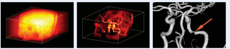
From left to right: X-ray rendering of magnetic resonance angiogram; filtering result using component tree techniques able to extract connected structures; and detail of the extracted structure. Images generated using the mtdemo program (http://www.cs.rug.nl/~michael/MTdemo/). |
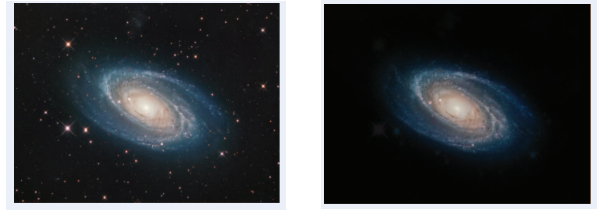
Right: spiral galaxy M81.
(credit: Giovanni Benintende). Left: filtered
result using k-flat connected filter approach (original paper: https://ieeexplore.ieee.org/document/5432219). Region-based approaches allow great suppression of the stars while preserving the edge details within the galaxy. |
In short:
- Connected component trees are very efficient hierarchical representations that can deal more efficient with region-based or object-based applications that the classical pixel-based processing,
- They have attractive properties to efficiently analyze, filter, extract specific structures in any data set.
Hierarchical Representations of 2-D Tera-Scale data sets
Gazagnes S., Wilkinson, M.H.F. Distributed Component Forests in 2-D: Hierarchical Image Representations Suitable for Tera-Scale Images. International Journal of Pattern Recognition and Artificial Intelligence, 2019
Context
When the evolution of image acquisition techniques, image sizes get larger and more complex to process efficiently. The hierarchical representations of these images, such as the component trees introduced above, also become larger, which makes them difficult to be stored or even used on modest compute servers, which typically can handle images up to few gigapixels (1 billion pixels). This is despite the attractive properties of these tree structures, that they form a
very efficient multi-scale representation which can represent all scales present in the image.
In a recent paper (2018), we extended and improved a new technique, called a Distributed Component Forest (DCF). The core idea is a divide-and-conquer approach: the image is first divided in smaller tiles, and we build and correct the local hierarchical representations of these tilesin a parallel manner such that processing the "forest"of these local trees yields the same result as if the a single tree representation was built for the whole data set. This new technique is particularly interesting as the Big Data era, as building a single tree for a very large data sets can be very computationally costly, and requires very specific computer servers. The DCF approach is an efficient approach to process very large data sets, in astronomy, remote sensing, or medical imaging.
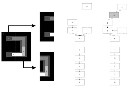
A simplified example of DCF construction. From left to right: the original image; the tiles after division; the local component trees for each tile; the final trees after having been corrected in a parallel manner.
|
The left figure shows a very simplified example of a DCF construction. The original image is divided in two tiles, for which the component trees are built individually. Because some structures span over the whole image, and hence are split in half due to the image division, these trees need to be corrected in parallel such that the missing information is shared between the processes. Note that only the information related to structures spanning over several tiles need to be exchanged. All structures fully contained within a single tile do not need to be corrected, because they don't share any pixels with other tiles. This correction is done using a distributed communication interface that exchange data chunks from one process to an other. The communication is optimized to avoid overload due to too many or too large messages. At the end of the process, the individual trees are corrected, such that their information have been updated (e.g the gray part in the right part of the left figure). Processing the two individual trees yield the same results as if we had only a single tree, but in that way, we reduce the memory footprint needed, and we improve the total computational time.
|
Example of DCF
Performance assessment
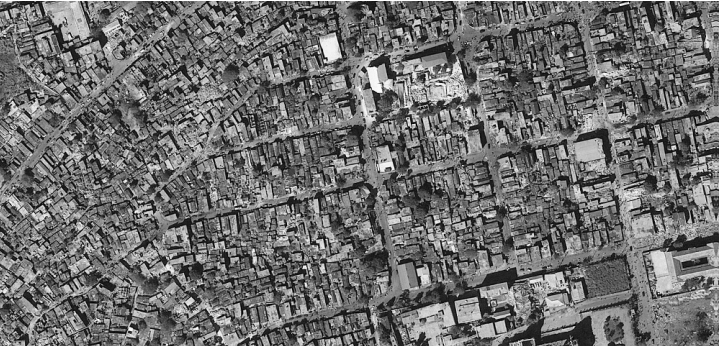
Cut into the remote sensing image of Haiti, 1.2 gigapixels.
|
To assess the performance of this method, we test it on several images, with different level of complexity. Typically, as the image gets larger, or as its dynamic range increases (the number of possible intensity levels), its processing becomes more difficult and complex. We tested our method by increasing the number of processes, such that the image is divided in N tiles, where N is the number of processes used. We report the processing time needed in each case, and the memory footprint. From this, we can compute the "speed-up" of the method, which is simply the ratio between the time it takes in the original case (1 process, no parallel processing), to the time it takes when we use N processes.
|
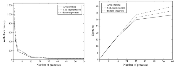
The figure above shows the computational time on the left, and the speed up on the right. As seen there, using multiple process largely improves the processing time needed to perform some filtering or analysis of its connected structures. When using one process, the computational time is between 800 and 1200 seconds (13 to 20 minutes) depending on the operation performed on the image. Using 16 processes already only require 60 seconds. The minimum time is 24 seconds and is obtained when using 64 processes (speed up of ~30). Additionally, while not showed here, the memory footprint (the amount of RAM needed typically) also decreases linearly with the number of processes. Hence this approach is very powerful to handle very large data sets, but is limited to low dynamic range images (see paper below for the extension of larger dynamic ranges).
In short:
- As image size gets larger, connected component trees become more complex to build and store, and hence require parallel, distributed approach that can lower the memory footprint and the computational time.
- The Distributed Component Forest in an approach that allows efficient parallel processing of very large images by dividing the original data sets in smaller chunks and building a forest of individual component trees that can be processed in a parallel manner.
Distributed Connected COmponent Filtering and ANalysis (DISCCOFAN)
Gazagnes S., Wilkinson, M.H.F. Distributed Connected Component Filtering and Analysis in 2-d and 3-d Tera-Scale datasets. IEEE Transactions on Image Processing 2021.
Context
This paper extends the previous DCF-2D code that enabled morphological analyses of objects and structures and large datasets.
This paper extends the previous DCF-2D code that enabled morphological analyses of objects and structures and large datasets.
In short:
- We extended the code to deal with 2D and 3D data sets using an hybrid approach that combines both MPI-based and threading-based parallelization
- The code scales better than any comparable approaches. We successfully ran the code on a 162 Gigavoxels dataset in 2 hours 20 minutes instead of the ~29 hours that would have been needed without parallel processing.
Parallel Attribute Computation for Distributed Component Forests
Gazagnes S., Wilkinson, M.H.F. Parallel Attribute Computation for Distributed Component Forests. 2022 IEEE International Conference on Image Processing (ICIP).
In short:
- We extended the code to enable posterior attribute computation in a parallel or distributed manner. This novel approach significantly reduces the computational time needed for combining several attribute functions interactively in Giga and Tera-Scale data sets.
